tickbound: timing GPU kernels from inside the SASS

GPU kernels are fast enough that the way you time them can be bigger than the thing you are timing. A kernel that runs for about 7 µs on the GPU can measure as 26 µs if the timer also catches the CPU launching it.

tickbound is the tool I built for my MSc research on GPU and host time synchronisation. It puts clock reads inside the compiled kernel, checks they landed where intended, and reports every number with a bound on how wrong it can be, together with the assumptions that bound rests on.

This post walks through it one diagram at a time.

The short version:

Timers are patched into the GPU machine code (SASS) after the compiler has run, so the compiler cannot move them. In straight-line code the kernel's own instructions stay bit-identical, and every build is checked for that.
A "sliding probe" gives the issue time of most instructions in a real kernel (129 of the 173 positions in one pass), and moved the median pass time by at most 4 cycles.
A chain of clock links puts events from eight A100s on one host clock, each GPU to within ±0.85 to 1.2 µs, and says plainly when that is not enough to prove an ordering.
I re-timed the kernels of a published SASS-reordering paper (CuAsmRL) on my own A100 rebuild. Its timing method varies by up to 1.33× between runs of some unchanged kernels, enough to cover its published gain on one kernel (fused_ff) but not its largest one (rmsnorm).
Issuing loads earlier, in batches, gives per-kernel median speed-ups of 1.2× to 3.0× on six real kernels.

Why I built it

I started tickbound for my MSc project: putting GPU events on the host's clock with a stated error, across several GPUs. Doing that properly needs timers inside the kernel whose position you can trust, which means checking them in the compiled SASS rather than in the source. The bracket method itself goes back to my final-year project at Sussex, which I wrote up here.

Along the way I looked at CuAsmRL (He and Yoneki, CGO 2025), which reorders SASS with reinforcement learning and reports 2 to 26 % speed-ups. Section 7 is what I found when I re-timed its kernels.

1. The pipeline

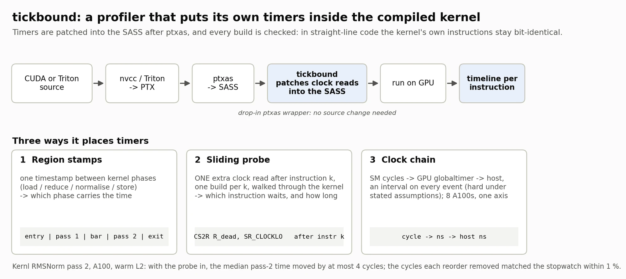
Pipeline: CUDA or Triton source, nvcc or Triton to PTX, ptxas to SASS, tickbound patches clock reads into the SASS, run on GPU, timeline per instruction. Below, three cards: region stamps, sliding probe, clock chain. — Where tickbound sits in the compile chain, and the three ways it places timers.

Reading the top row. A kernel starts as CUDA or Triton source. nvcc or Triton turns it into PTX, NVIDIA's portable assembly. ptxas then turns PTX into SASS, the machine code the GPU actually runs. The two blue boxes are tickbound's part: it patches clock reads into that final SASS, runs it, and turns the readings into a timeline per instruction.

Because it acts after ptxas, the compiler never sees the timers and cannot reorder around them. It runs as a drop-in ptxas wrapper, so it needs no changes to the kernel's source. It does need spare registers (the RMSNorm probe build below went from 32 to 66 registers, which can cut occupancy), and in kernels with branches it has to rewrite branch offsets, so "bit-identical" holds for straight-line code like the pass shown here. The timings in this post were placed by per-kernel scripts; the automatic version is built but not yet validated on a GPU.

Reading the three cards. Each card is one way of placing timers, with a one-line picture of what gets inserted:

Region stamps put one timestamp, a GPU-timer read paired with a cycle-counter read, between the kernel's phases (load, reduce, normalise, store). They answer: which phase carries the time?
The sliding probe adds one extra clock read after instruction k, in a separate build for each k, and walks it through the kernel. It answers: which instruction waits, and for how long?
The clock chain converts SM cycles to the GPU's nanosecond timer and then to the host clock, giving an interval at every step that is a hard bound under the assumptions in section 5. It puts different SMs and different GPUs on one axis.

The footer gives the two checks the RMSNorm probe passed (pass 2, A100, warm L2): with the probe in, the median pass-2 time moved by at most 4 cycles, and the cycles each reorder removed matched an independent stopwatch to within 1 %.

The ingredients for this exist already (NVBit, CUPTI). What tickbound adds is putting them together so that every number comes with a stated bound.

2. Where the clock read goes decides what you measure

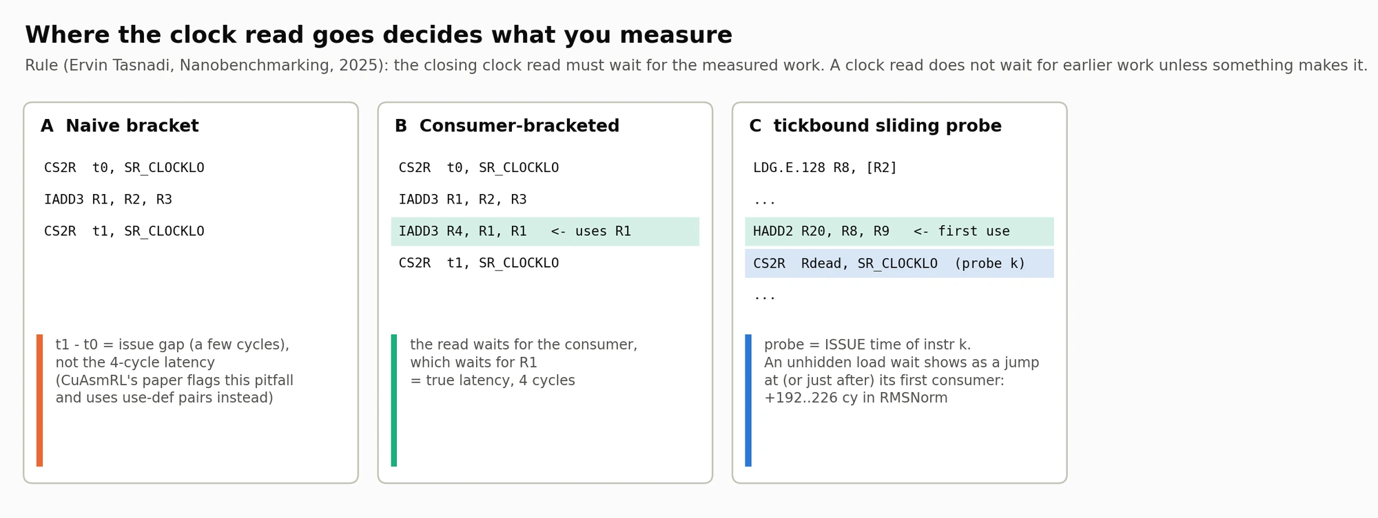
Three panels: A, a naive bracket measures only the issue gap of IADD3, not its 4-cycle latency. B, a consumer-bracketed read waits for a dependent instruction and measures the true latency. C, the sliding probe reports issue time, and an unhidden load wait shows as a jump at or just after its first consumer. — Three ways to bracket an instruction with clock reads. Only the placement changes; the result changes completely.

The rule behind this figure comes from Ervin Tasnadi's Nanobenchmarking post: the closing clock read must wait for the work being measured. On a GPU a clock read does not wait for earlier instructions unless something forces it to.

Panel A, the naive bracket. Read the clock, issue IADD3, read the clock again. The second read does not wait for the add to finish, so t1 - t0 is only the issue gap between the clock reads, a few cycles, not the add's 4-cycle latency. CuAsmRL's paper flags this same pitfall and uses use-def pairs instead.

Panel B, consumer-bracketed. Insert an instruction that uses the result (the green line, IADD3 R4, R1, R1) before the closing read. That consumer cannot start until R1 is ready, and the closing read comes after the consumer, so now the bracket covers the true 4-cycle latency.

Panel C, the sliding probe. tickbound does not try to make the probe wait. The probe (blue line) reports when instruction k was issued, and the hardware's own dependency tracking does the rest. When a load's data has not arrived yet, its first consumer stalls, and the issue time jumps there or, if the probe cannot be placed right after it, one or two instructions later. In RMSNorm those jumps are 192 to 226 cycles: the part of each L2 round trip that the instructions in between could not hide.

So tickbound's closing reads go after a consumer, or after a barrier followed by a memory instruction (section 3 shows why the barrier alone is not enough), and the probe is read as issue time, never as latency.

3. What the timers look like in real SASS

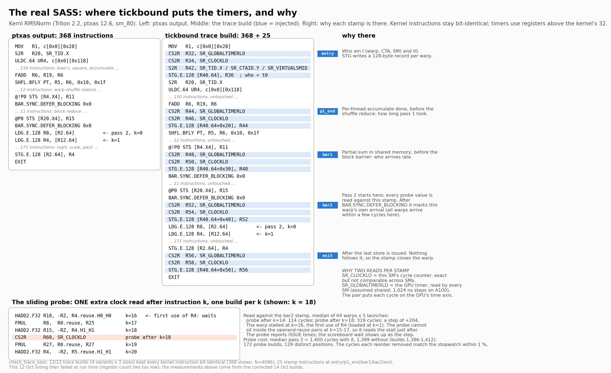
SASS of Kernl RMSNorm: 368 ptxas instructions on the left, the trace build with 25 injected instructions highlighted in blue in the middle, and on the right the reason for each stamp: entry, p1_end, bar1, bar2 and exit. Below, the sliding probe build after instruction 18, with the first use of R4 at instruction 16. — Kernl's RMSNorm, compiled by Triton 2.2 and ptxas 12.6 for the A100 (sm_80). Left: what ptxas produced. Middle: the trace build. Right: why each stamp is there.

This is not a sketch. It is the real SASS of a Triton RMSNorm kernel, before and after tickbound.

Left column: ptxas output, 368 instructions. Middle column: the trace build, the same 368 instructions plus 25 injected ones, highlighted in blue. Every original line is unchanged. The timers use registers above the 32 the kernel already uses, so they cannot overwrite its data.

Right column: why each stamp sits where it does.

entry records who this warp is (warp, block, SM) and its start time, and writes a 128-byte record per warp.
p1_end sits after the per-thread accumulate and before the shuffle reduce: how long pass 1 took.
bar1 sits before the block barrier: which warps arrive late.
bar2 marks the start of pass 2, and every probe value is measured against it. It sits right after BAR.SYNC.DEFER_BLOCKING, and that form of barrier lets a clock read issue as soon as this warp arrives, before the others have. So bar2 marks each warp's own arrival rather than the block's release. In this kernel the difference is small; reading the true release needs a memory instruction between the barrier and the clock read.
exit comes after the last store is issued and closes the warp.

Why two clock reads per stamp. SR_CLOCKLO is the SM's own cycle counter: exact, but every SM starts it at a different value, so two SMs cannot be compared directly. SR_GLOBALTIMERLO is the GPU timer, which every SM reads; tickbound assumes it is one shared timer (on the A100 it steps every 1,024 ns). Reading both puts every cycle on the GPU's time axis, and the host sync (section 5) puts that axis on the host's clock.

The bottom panel shows one probe build: a CS2R placed right after instruction 18. The warp actually stalls two instructions earlier, at instruction 16 (HADD2.F32 R18, -RZ, R4.reuse.H0_H0), the first use of R4, which waits for the load at instruction 1. The probe cannot sit inside the operand-reuse pairs at instructions 15 to 17, so the readings either side of the stall are instruction 14 at 114 cycles and instruction 18 at 319 (median of 64 warps × 5 launches): a step of +204 cycles, the part of that load's L2 round trip nothing hid.

The cost of looking is small. The median pass-2 time is 1,400 cycles with the probe in and 1,399 without (individual probe builds ranged from 1,386 to 1,412). It took 172 builds to slide the probe through the 173 instructions of pass 2; because it skips reuse pairs, that gives 129 distinct positions for this kernel.

The check at the bottom confirms that all 12 trace builds (4 variants × 3 row sizes) kept every kernel instruction bit-identical, including the 368 shown. This particular listing is from 12 Oct, and it then failed at run time because its register count was two too low; the measurements above come from the corrected 14 Oct builds.

4. The sliding probe as a timeline

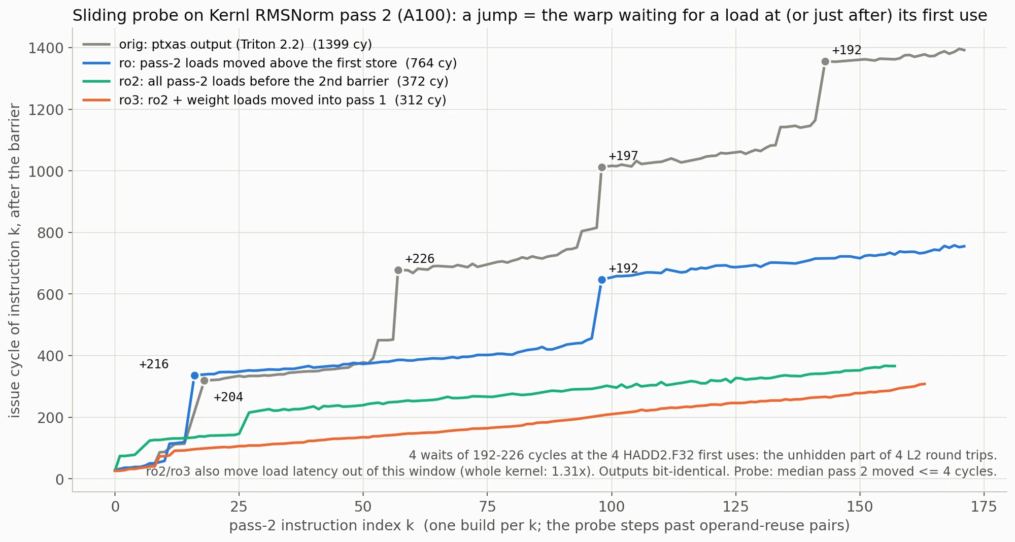
Line chart of issue cycle against pass-2 instruction index for Kernl RMSNorm on an A100. The grey original line climbs to 1,399 cycles with four jumps of 192 to 226 cycles. The ro variant (blue) reaches 764 cycles with two jumps; ro2 (green) and ro3 (orange) are flat, at 372 and 312 cycles. — Kernl RMSNorm pass 2 on an A100. Each jump is the warp waiting for a load at, or just after, its first use.

How to read it. The x-axis is the instruction index k in pass 2; each point is a separate build with the probe right after instruction k (or the next instruction it can sit after). The y-axis is when that instruction issued, in cycles after the bar2 stamp. A steady slope means the warp is issuing; a vertical jump means it stood still.

The grey line is the kernel as ptxas compiled it: 1,399 cycles, with four jumps of 192 to 226 cycles. Each one sits on, or one or two instructions after, one of the four HADD2.F32 instructions that first use a loaded weight vector. Each load is issued a few instructions before its first use, so each jump is the part of an L2 round trip that those instructions could not hide.

The coloured lines are three variants:

ro (blue, 764 cycles): the pass-2 loads moved above the first store. Two of the four waits disappear.
ro2 (green, 372 cycles): all pass-2 loads moved before the second barrier, so they are in flight during the block reduction. All four waits disappear.
ro3 (orange, 312 cycles): ro2 plus the weight loads moved up into pass 1, which also removes the smaller steps that remain.

The outputs are bit-identical in every variant. Note that ro2 and ro3 move part of the load latency before the bar2 stamp, outside this window, so the whole kernel gains less than this chart suggests: 1.31× for this case (figure 6).

I had predicted those four waits from reading the SASS. A total kernel time only shows that something is slow; the probe timeline confirmed them one instruction at a time, with a cycle count for each.

5. From a warp's cycle to the host clock

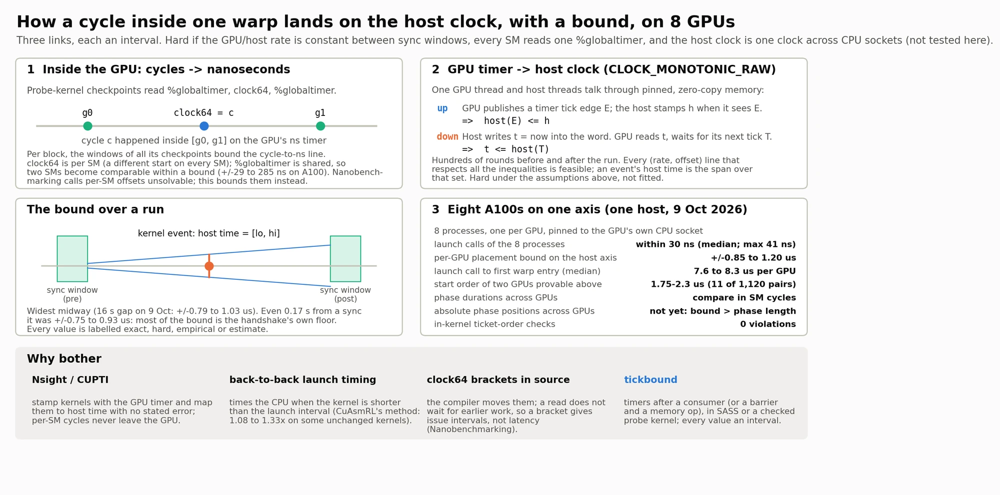
Diagram of the clock chain: link 1 converts cycles to GPU nanoseconds with g0, clock64, g1 checkpoints; link 2 bounds the GPU timer against the host clock through up and down handshakes; a panel shows the bound over a run between two sync windows; link 3 lists the results for eight A100s; a final row compares Nsight and CUPTI, back-to-back launch timing, clock64 brackets in source, and tickbound. — Three links from a cycle inside one warp to the host clock. Each link is an interval rather than a point.

The bounds in this figure are hard under three assumptions, listed at the top: the GPU timer and the host clock keep a constant rate ratio between two sync windows; every SM reads the same %globaltimer (checked only to about 0.25 to 0.5 µs on the A100); and the host clock is one clock across both CPU sockets, which this run did not test. Every value in the figure is labelled exact, hard, empirical or estimate.

Link 1, inside the GPU: cycles to nanoseconds. In the eight-GPU probe kernel, each checkpoint reads the global timer, then the cycle counter, then the global timer again (g0, c, g1). So cycle c happened somewhere inside [g0, g1] on the GPU's nanosecond timer. Across all the checkpoints in a block, those windows bound the cycle-to-nanosecond line. That makes two SMs comparable within a bound, ±29 to 285 ns per run on the A100. Nanobenchmarking calls per-SM counter offsets unsolvable, and tickbound does not solve them either; it bounds them instead. (The RMSNorm stamps in section 3 use two reads, timer then cycles.)

Link 2, GPU timer to host clock. One GPU thread and the host talk through pinned, zero-copy memory, in two directions:

up: the GPU publishes a tick edge E of its timer, and the host stamps h when it sees it. So host(E) ≤ h.
down: the host writes t = now. The GPU reads it and waits for its next tick T. So t ≤ host(T).

Hundreds of these rounds run before and after the kernel. Every rate-and-offset line that satisfies all the inequalities is feasible, and an event's host time is the span over all of them: a hard bound under the assumptions above, not a fitted line.

The bound over a run (bottom left). The bound is widest midway between two sync windows: ±0.79 to 1.03 µs over a 16 s gap on 9 Oct. Even 0.17 s from a sync it was ±0.75 to 0.93 µs, so most of the bound is the handshake's own floor rather than the distance from the sync.

Link 3, eight A100s on one axis (bottom right), one host, 9 Oct 2026:

the eight processes, one per GPU and pinned to that GPU's own CPU socket, issue their launch calls within 30 ns of each other (median; max 41 ns);
each GPU is placed on the host axis to within ±0.85 to 1.20 µs;
from launch call to first warp entry takes a median of 7.6 to 8.3 µs per GPU (single launches 7.1 to 10.2 µs); with bounds of about ±1 µs, the GPUs cannot be told apart on this;
the start order of two GPUs can be proven only when they start more than 1.75 to 2.3 µs apart under the conservative rule (the gap must exceed the sum of both bounds), which happened in 11 of 1,120 pairs. With exact per-instant intervals the threshold drops to about 1.66 µs and 20 pairs. Five of the 11 strict proofs are cross-socket pairs, so they rely on the untested one-host-clock assumption;
phase durations compare across GPUs in SM cycles, but absolute phase positions cannot yet, because the bound is bigger than a phase;
in-kernel ticket-order checks: 0 violations.

The "why bother" row compares the usual options. Nsight Systems and CUPTI stamp each kernel with the GPU timer (in 32 ns steps while a profiler is attached) and map it to host time with no stated error; per-SM cycles never leave the GPU. Timing back-to-back launches measures the CPU whenever the kernel is shorter than the launch interval. clock64 brackets in source code get moved by the compiler, and measure issue intervals rather than latency. tickbound's timers sit after a consumer, or after a barrier plus a memory instruction; they are either patched into the SASS (the RMSNorm runs) or written into a purpose-built probe kernel and checked in its SASS (the eight-GPU run), and every value is an interval on one host axis.

6. Eight GPUs on one clock

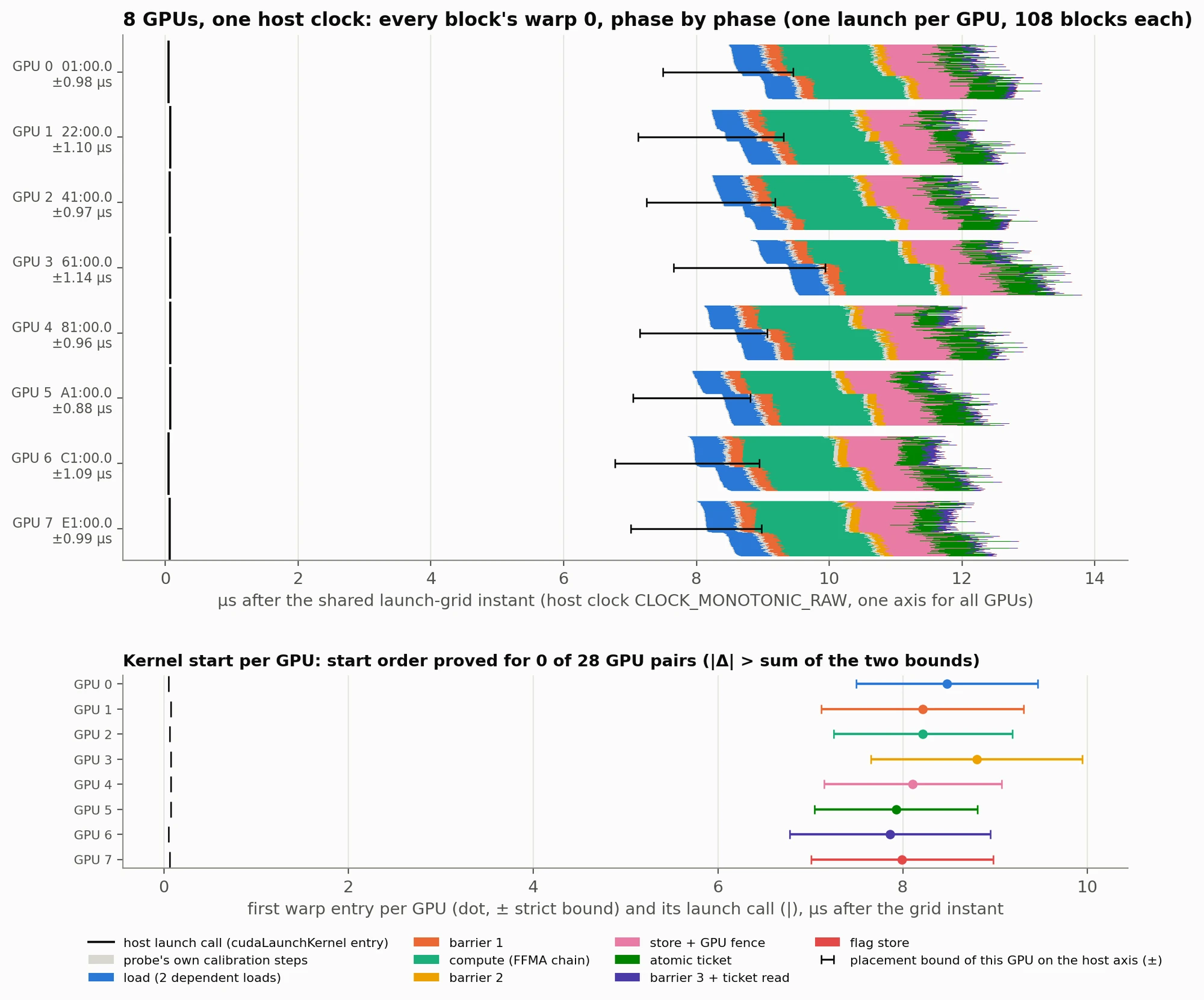
Timeline of eight A100 GPUs on one host clock, every block's warp 0 drawn as a coloured strip by phase, with a black placement bound per GPU. Below, the kernel start per GPU with error bars; the start order is proven for 0 of 28 GPU pairs. — tickbound's own probe kernel, one launch per GPU, 108 blocks each, every block's warp 0, all on the host's CLOCK_MONOTONIC_RAW.

This run uses tickbound's own probe kernel rather than a real workload: two dependent loads, an FFMA chain, barriers, a store and fence, and an atomic ticket, with a checkpoint at every phase boundary.

How to read the top panel. Each row is one GPU, labelled with its PCI address and its placement bound (between ±0.88 and ±1.14 µs in this run). Time runs left to right in microseconds after the shared instant all eight processes launched. The thin black mark near zero is each process's launch call. Each GPU's band is made of 108 thin strips, one per block, coloured by phase: the two dependent loads (blue), barrier 1 (orange), the FFMA compute chain (green), barrier 2 (yellow), the store and GPU fence (pink), the atomic ticket (dark green), barrier 3 and the ticket read (purple). The black bar across each band is how far that whole band could slide on the host axis.

The bottom panel zooms in on one question: which GPU started first? Each dot is a GPU's first warp entry, with its bound. In this run every pair of bounds overlaps, so under the conservative rule the start order is proven for 0 of 28 pairs.

That is an honest result, and the main reason I trust the tool. It draws the timeline, and it also tells you which conclusions the timeline cannot support yet. Within one warp, phase durations are exact in SM cycles. Blocks on different SMs of one A100 line up to within about ±0.03 to 0.29 µs, and different GPUs to about ±1 µs, so two kernels on different GPUs can only be ordered when they start roughly 1.7 µs or more apart.

7. Re-checking CuAsmRL

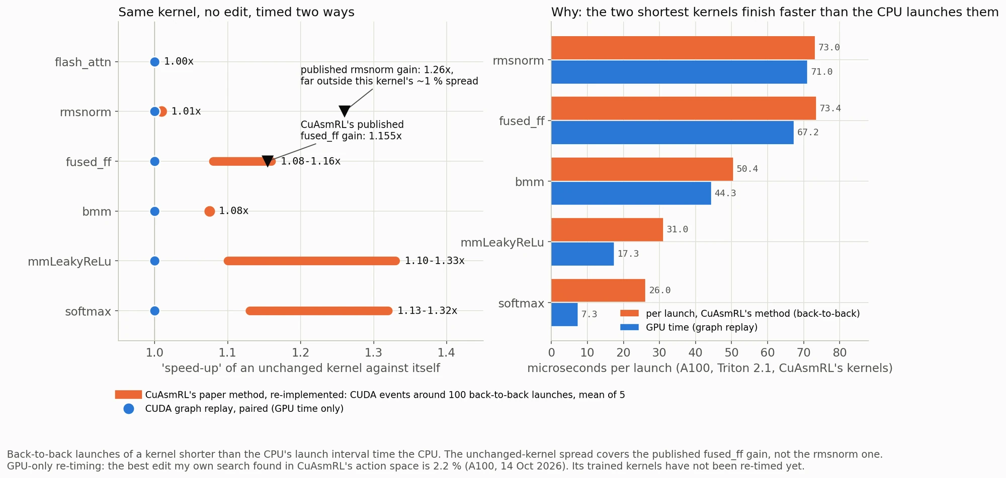
Left: unchanged kernels timed against themselves. With CuAsmRL's back-to-back timing method, four of the kernels show apparent speed-ups of 1.08 to 1.33 times, a band containing the published fused_ff gain of 1.155 times; rmsnorm and flash_attn stay within about 1 percent, far below the published rmsnorm gain of 1.26 times. Right: per-launch time under that method against GPU time for five kernels. — The same unchanged kernels, timed two ways. A100, CuAsmRL's own kernels and Triton version (2.1).

All of this ran on an A100 with CuAsmRL's own kernels, Triton version (2.1) and benchmark helper, with Triton's bundled ptxas 12.1 (the paper used 12.2).

The left panel asks: if you time a kernel against itself, with no edit at all, what "speed-up" do you see? Blue dots are GPU-only timing (CUDA graph replay, paired), and they sit at 1.0, as they should. Orange is CuAsmRL's timing method as its paper describes it, which I re-implemented: one CUDA event pair around 100 back-to-back launches, averaged over 5 runs. For four of the kernels (softmax, mmLeakyReLu, bmm and fused_ff) it reports 1.08 to 1.33× between two runs of the same code. The black triangle on fused_ff is CuAsmRL's published 1.155× gain on that kernel, and it lands inside the band an unchanged kernel produces. On rmsnorm and flash-attention, though, the same method is steady to about 1 %, so its largest published gain, 1.26× on rmsnorm, is far outside the noise.

The right panel shows one cause, for the two shortest kernels. Orange is the per-launch time under that method, blue is the GPU time. For softmax it is 26 µs per launch against 7.3 µs of GPU time: the CPU cannot launch as fast as the GPU finishes, so the average over back-to-back launches measures the CPU's launch rate. For softmax and mmLeakyReLu the per-launch time is 1.8 to 3.6× the GPU time. For the three longer kernels it is within about 15 %, so launch overhead does not explain the spread on bmm and fused_ff.

Three findings:

Timing. On four of the six kernels, this timing method varies by 8 to 33 % between runs of unchanged code, which covers the published fused_ff gain. It does not explain the rmsnorm result. I have not yet re-timed CuAsmRL's own trained kernels, so this says nothing about whether their gains are real, only that numbers from this method need paired GPU-only timing before they can be trusted.
Correctness. Under my re-implementation of its legality masks, 178 of 320 random episodes of up to 32 moves on rmsnorm changed the output bytes. My own stricter checker also passed 6 moves that changed outputs. So static legality is not enough on its own: outputs have to be compared, as CuAsmRL also does by testing.
Search. Inside its action space, with paired GPU-only timing and byte checks, the largest gain my own search found is 2.2 % (bmm), and most kernels show none. That is the best my search found, not an upper bound.

Correction. An earlier version of my LinkedIn post said CuAsmRL's latency table came from naive clock brackets. That was wrong: the paper identifies that pitfall and derives its Table 1 from use-def pairs (IADD3 = 4 cycles). I apologised to the authors.

8. What issuing loads earlier is worth

So moving loads is not worthless. The question is which move, and how you measure it.

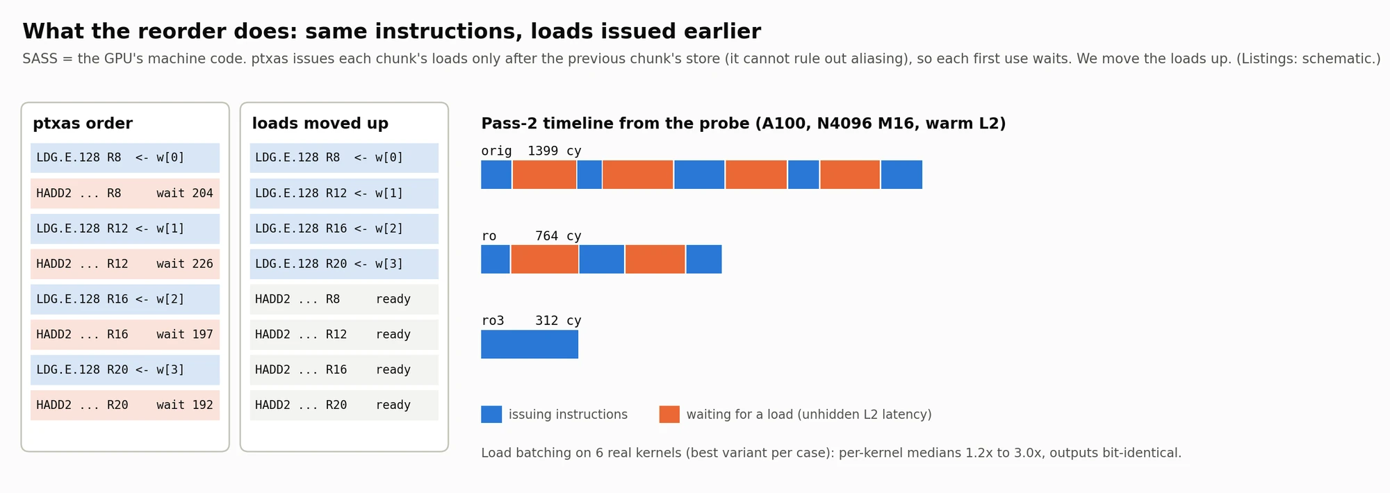
Schematic listings: in ptxas order each weight load is followed by its use, which waits 204, 226, 197 and 192 cycles; with the loads moved up, every use is ready. Right: pass-2 timelines of 1,399, 764 and 312 cycles, blue for issuing and orange for waiting. — Same instructions, loads issued earlier. RMSNorm pass 2 on an A100 (N = 4096, M = 16, warm L2). The listings are schematic; figure 9 shows the real order.

Reading the left two columns. In ptxas's order, each chunk's loads sit right after the previous chunk's store, because ptxas cannot prove the output does not alias the inputs (Triton emits no noalias). Each first use then waits 204, 226, 197 and 192 cycles: the part of the L2 round trip that the few instructions in between cannot hide. Moving the loads up is legal here only because both real callers allocate a fresh output, and outputs are byte-compared to check it.

Reading the bars on the right. Blue is time spent issuing instructions, orange is time spent waiting for a load. The original pass is mostly orange: 1,399 cycles. Moving the loads above the first store gives 764. The ro3 variant gives 312, with almost no waiting left, partly by moving load latency before the timed window. The output is bit-identical. This is done at PTX level through the ptxas wrapper, not by editing SASS by hand.

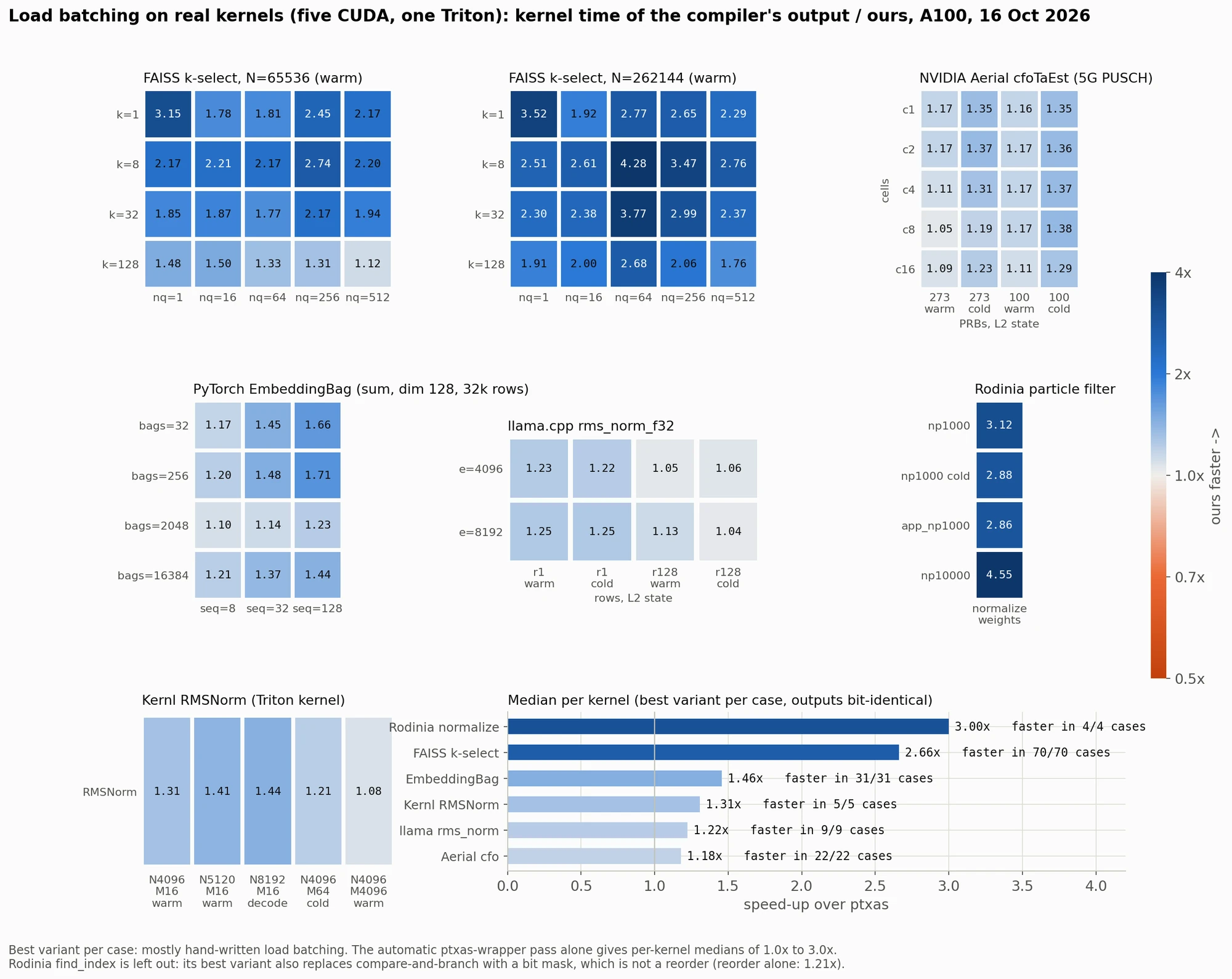
Heatmaps of speed-up over the compiler for FAISS k-select at two sizes, NVIDIA Aerial cfoTaEst, PyTorch EmbeddingBag, llama.cpp rms_norm, Rodinia normalize_weights and Kernl RMSNorm, with a bar chart of the median per kernel. — Load batching on real kernels (five CUDA, one Triton), A100, 16 Oct 2026. Each cell is the compiler's kernel time divided by ours.

How to read the heatmaps. Each panel is one real kernel, swept over its own parameters: k and the number of queries for FAISS k-select, cells and PRBs for NVIDIA Aerial's 5G uplink frequency- and timing-offset estimator (cfoTaEst), bags and sequence length for PyTorch's EmbeddingBag, and so on. "Warm" and "cold" are the state of the L2 cache. Each cell is the compiler's kernel time divided by ours, so anything above 1.0 (blue) means our build is faster. Darker blue is a bigger win, up to 4.55× on one Rodinia case.

These are the best variant per case, and most of those are hand-written load batching in the kernel source; the automatic ptxas-wrapper pass alone gives per-kernel medians of 1.0× to 3.0×. The bar chart at the bottom right gives the median per kernel, and in every case measured the best variant was faster:

Rodinia normalize_weights: 3.00×
FAISS k-select: 2.66×
PyTorch EmbeddingBag: 1.46×
Kernl RMSNorm (the Triton kernel): 1.31×
llama.cpp rms_norm: 1.22×
NVIDIA Aerial cfoTaEst: 1.18×

All outputs are bit-identical to the compiler's. Rodinia find_index is left out on purpose: its best variant also replaces compare-and-branch with a bit mask, which is not a reorder (the reorder alone gives 1.21×).

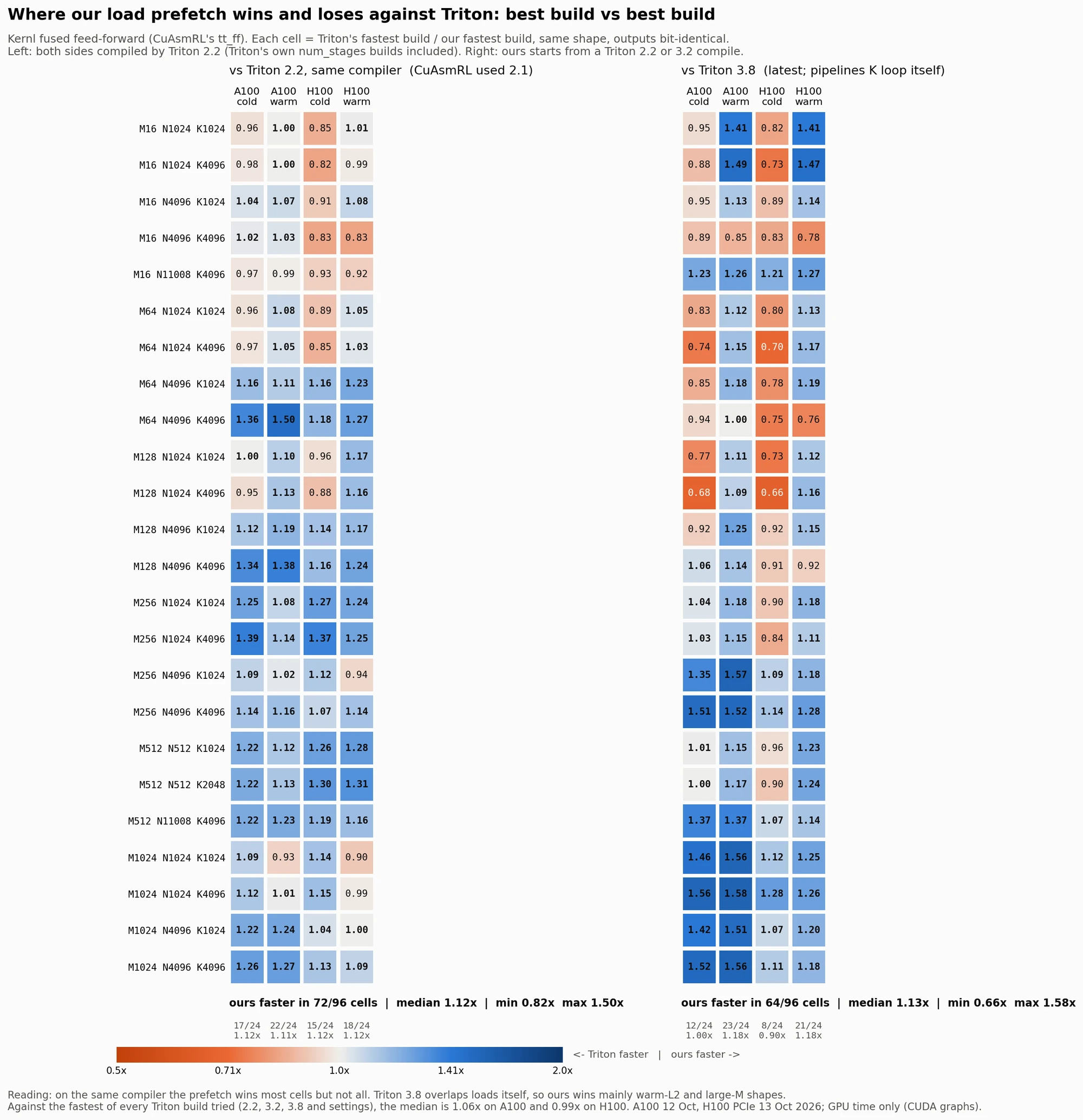
Two heatmaps for CuAsmRL's fused feed-forward over 24 shapes on A100 and H100, cold and warm L2. Left, against Triton 2.2 on the same compiler: ours faster in 72 of 96 cells, median 1.12. Right, against Triton 3.8: ours faster in 64 of 96 cells, median 1.13, with orange losses on cold-L2 small-M shapes. — CuAsmRL's fused feed-forward, Triton's best build against our best build. Blue means ours is faster, orange means Triton is.

The last figure is the fairest test I could set up. For CuAsmRL's fused feed-forward kernel, across 24 matrix shapes (rows), on the A100 and H100 with a cold or warm L2 (columns), it compares Triton's fastest build with ours. Here the change is a prefetch: each loop iteration loads the next iteration's data.

Left, same compiler (Triton 2.2; CuAsmRL used 2.1). Both sides are compiled by Triton 2.2, and Triton's own num_stages settings count on its side. Ours is faster in 72 of 96 cells, median 1.12× (range 0.82 to 1.50×).

Right, against Triton 3.8, the current version, which pipelines its loads itself. Ours (starting from a Triton 2.2 or 3.2 compile) is faster in 64 of 96 cells, median 1.13× (range 0.66 to 1.58×). It helps mainly with a warm L2 and large M; with a cold L2 and small M, Triton wins on both GPUs, by up to 1.5×. Against the fastest of every Triton build I tried, the median is 1.06× on the A100 and 0.99× on the H100.

The orange cells are part of the result, not something to hide.

What I take from this

Measure on the GPU, not around it. For short kernels, back-to-back launch timing measures the CPU. Graph replay with paired runs, or timers inside the kernel, measure the GPU.
Put a bound on every number, and say what it assumes. A timeline is only as good as the claims it can support. "0 of 28 pairs provable" is more useful than a confident picture that might be wrong.
Compare like with like. A new compiler version can look like an optimisation. Keep the compiler fixed, and include its own tuning knobs on its side.
Look per instruction. The four waits in RMSNorm were invisible in a total kernel time. Predicted from the SASS, they were confirmed one instruction at a time by the probe, and the fix was simple.

What's next

This is the groundwork for my MSc project on GPU and host time synchronisation. Next: test the one-host-clock assumption across CPU sockets, tighten the cross-GPU bound until kernel order across GPUs becomes provable, validate the automatic placement on a GPU, and re-time CuAsmRL's trained kernels with paired GPU-only timing.

The write-up and run data (findings, CSVs, SASS) are here. Raw traces and the tool are available on request. If you work on kernels or compilers, I'd like to hear where this breaks.